by John Middendorf
The following procedure uses GIS to find suitable
sites for a winery.
Seven criteria are identified,
namely:
- Outside the floodplain and more than 100 meters from a stream.
- Agricultural or undeveloped landuse.
- Flat land or 112-337 slope aspect.
- Average maximum windspeed of less than 25 mph.
- Average minimum temperature of greater than 35 degrees.
- Soil depth between 31 and 72 inches.
- 1.5 to 3 soil drainage values.
We will use the following data:
- Climate point data
- Soil depth point data
- Floodplain polygon
- Landuse polygon
- Hydro line data
- Elevation raster grid.
The initial steps in this project are to convert all data into raster format for analysis. Using ESRI's spatial analyst, we set the ANALYSIS CELL SIZE to 10m for all future conversions.
For the Landuse, we first DISSOLVED the landuse polygons into the four discrete classes, converting 80 features into four features. Then we converted the vector shapefile into raster format using SPATIAL ANALYST>CONVERT>FEATURES TO RASTER. We also converted the floodplain vector shapefile to raster format using this command.
Using the elevation raster grid, we used two commands in spatial analyst: HILLSHADE and ASPECT to create two new raster grids.
Next we created four raster grids from the climate and soils point data, using the command: SPATIAL ANALYST>INTERPOLATE TO RASTER>INVERSE DISTANCE WEIGHTED, which creates values based on proximity to a known point data. We used a 4th power relationship (higher powers mean that farther away points have less influence on the interpolated values).
The next step was to create buffered regions around the hydro line shapefile. Again we used spatial analyst since we were looking for a raster result, using SPATIAL ANALYST>DISTANCE>STRAIGHT LINE. This gave us the 100m boundary to rivers and creeks.
Below are the rasters created:
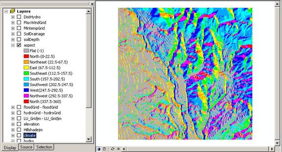
Above: Aspect unclassified raster grid.
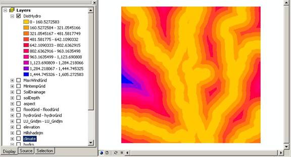
Above: Distance to hydro unclassified raster grid.
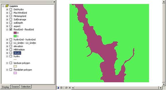
Above: Floodplain raster grid.
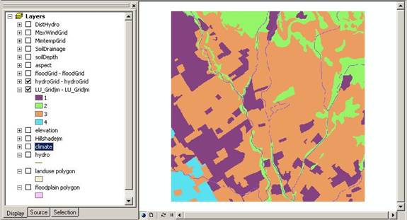
Above: Land use unclassified raster grid.
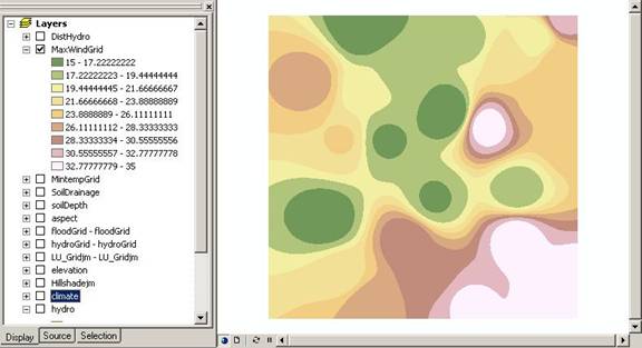
Above: Maximum wind speed unclassified raster grid.
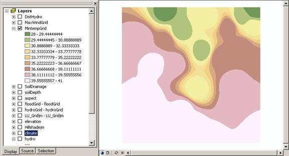
Above: Minimum temperature unclassified raster grid.
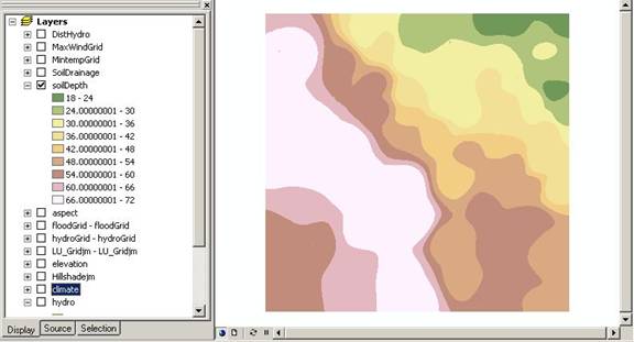
Above: Soil depth unclassified raster grid.
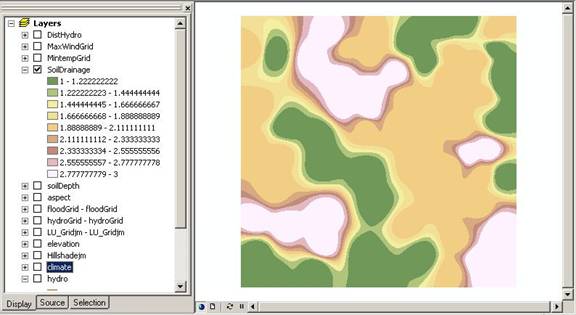
Above: Soil drainage unclassified raster grid.
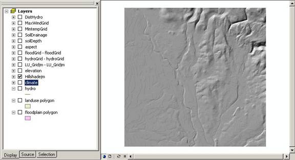
Above: Hillshade raster grid.
With everything now in raster format, we set about reclassifying the rasters to suit our criteria, using SPATIAL ANALSYT>RECLASSIFY. Zeros were given to regions outside the criteria, and the value 1 was given to suitable criteria regions. This enabled us to simplify finding the suitable regions by using SPATIAL ANALYST>RASTER CALCULATOR, by multiplying all raster together:
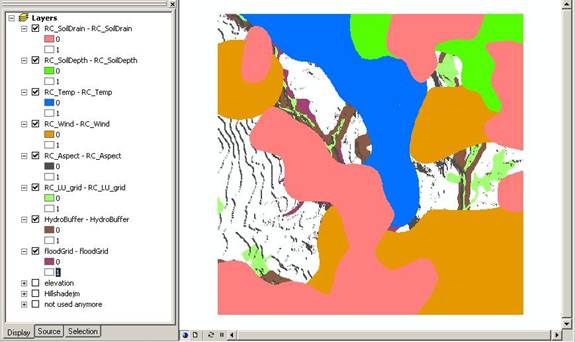
Above: Reclassified criteria rasters, with unsuitable areas colored, uncolored areas are the suitable areas.
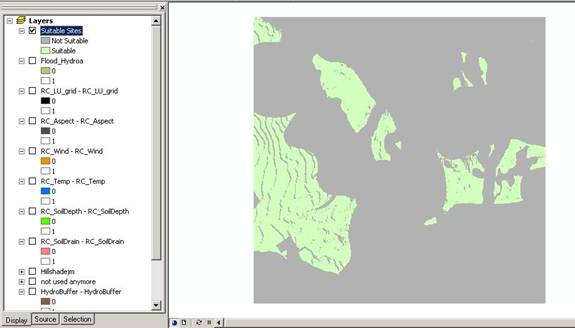
Above: Result after using the Spatial Analyst raster calculator to combine all unsuitable areas into one resulting raster output grid.
Note that after a raster calculation, the result needs to be saved using the MAKE PERMANENT command by right clicking the layer.
Finally, we compiled our final map showing suitable sites by using the hillshade layer as a base for visual clarity, then overlaying a 66 percent transparent flood plain, the hydro layer, and the suitable sites (also partially transparent) on top:
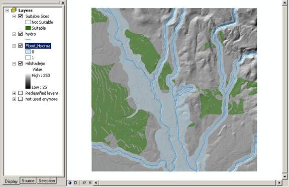
Above: final map showing suitable sites in green.
FINAL PRESENTATIONS
For the final layout, I made two versions, one
showing only
the suitable sites, and one with six additional views showing the
criteria
used: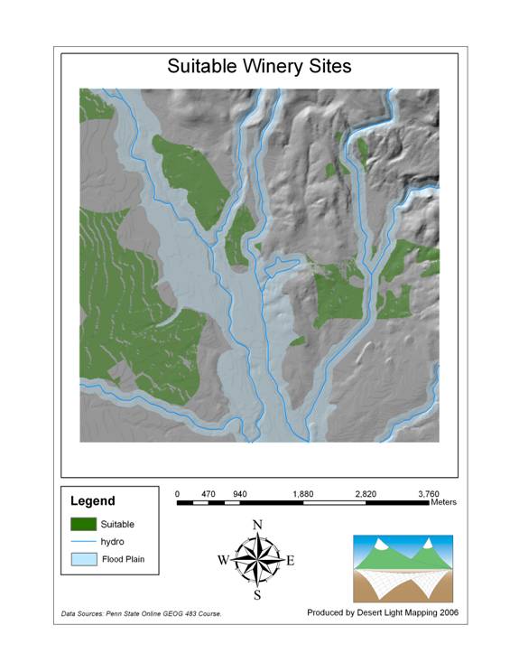
Above: Final Layout showing suitable winery sites.
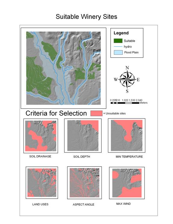
Above: Suitable winery sites with additional data views showing the criteria used to determine suitable sites.
In this map, 1295.3 acres of suitable land is shown, calculated by knowing the number of cells (52422, found in the attribute data) and the cell size (100 square meters), then multiplying the number of square meters by 10.7639 to get square feet, then dividing by 43,560 to get number of acres.
Finally, the land must be on private land. Using a process we became familiar with above, the layer was rasterized and classified into public and private and multiplied with the existing raster suitable layer:
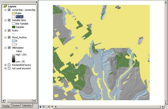
Above: Rasterized public/private layer added to the map.
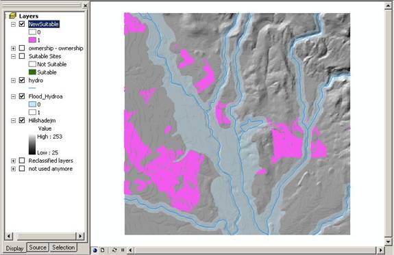
Above: after final spatial analyst calculation showing new suitable areas in magenta.
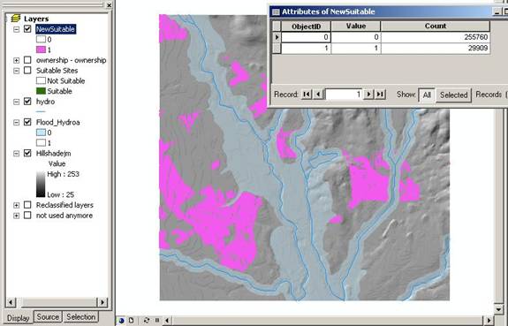
Above: the number of cells suitable (value =1) of the final suitable region.
SUITABLE ACREAGE LOST DUE TO CONSIDERATION ON PRIVATE LAND
With 29909 cells in the final suitable region, this correlates to 739.4 acres. Thus, 556 acres were lost due to the private land criteria (1295.3 acres minus 739.4 acres).
RESOLUTION OF DATA
With higher resolution data (e.g. cell size smaller than 10m), the analysis results could have been significantly different. Not only would the boundary of each criteria’s suitable regions be either larger or smaller than what was calculated here, but regions within each suitable (or unsuitable) region could have been reversed. This would likely be most significant for the Aspect layer, because of the large number of individual regions.
For the point data that was interpolated, the cell size also affect the results, though the factor of four used in the inverse weighted method probably had a greater influence. The grid size was probably least significant in the buffered layers (Flood plain and hydro) as a maximum of 10m error would be involved only on the boundary in these cases. The cumulative effect of the land use regions using a 10m grid (since there is significant total boundary length of all the divided parcels) could have been significant by the grid size.